TOC fit
To fit TOC data with pdom, one of the multi-species models must be selected:
- incremental
- fragmentation
- excess bonds
For this example, we will use incremental. The model for the desorption constant \(k_{\mathrm{ads}}\) is always weak when a TOC experiment is fitted.
The generation of the config file example_toc_fit.ini is again carried out with pdom.config.
Lines with require user input are highlighted in yellow.
$ pdom.config
ID of the system (avoid spaces): example_toc_fit

Should data be fitted to the simulation?
	1: fit
	2: just simulation
Your choice: 1

What kind of experiment was conducted?
	1: Adsorption-Desorption
	2: Degradation
	3: TOC
Your choice: 3

How can you identify the initial molecule?
	1: chemID (https://pubchem.ncbi.nlm.nih.gov)
	2: name
Your choice: 1
Molecule: 4139
Found methylene blue cation (C16H18N3S+)

What is the catalyst concentration?
  the allowed unis are: g/m^3, g/L, mg/L
Value: 2.5 g/L

What is the catalyst surface area?
  the allowed unis are: m^2/g, cm^2/g
Value: 56 m^2/g

What is the overall volume?
  the allowed unis are: m^3, L, cm^3, mL
Value: 1 L

How long should the simulation be?
  the allowed unis are: h, min, s
Value: 6 h

Which split model should be used?
	1: incremental
	2: fragmentation
	3: excess_bonds (slow)
Your choice: 1

Is the system in equilibrium (dark)?
	1: Yes
	2: No
Your choice: 1

Which parameter should be fitted?
	1: k_reac
	2: beta_1
Your choice: 2

What is the adsorption constant?
  the allowed unis are: m/s
Value: 3.0E-9 m/s

What is the desorption constant?
  the allowed unis are: 1/s
Value: 6.8E-3 1/s

What is the reaction constant?
  the allowed unis are: 1/s
Value: 6.8E-2 1/s

What is concentration in the solution?
  the allowed unis are: molecule/m^3, molecule/L, mol/m^3, mmol/L, M, mol/L, mo/mc, g/L, mg/L, g/m^3
Value: 0.069 mmol/L
After the config is generated, the experimental data set is created.
In this example, values published by Houas (2001) [Houas2001] will be used.
{
  "time_series": [
    [0, 60, 120, 180, 360],
    [12.6, 8.8, 6.78, 4.1, 2.77]
  ],
  "time_series_meta": [
    {
      "unit": "min",
      "type": "t"
    }, {
      "unit": "mg/L",
      "type": "toc"
    }
  ]
}
With both files prepared, pdom can be started.
$ pdom example_toc_fit.ini --data example_toc_fit.json
Start fitting to toc
   Iteration     Total nfev        Cost      Cost reduction    Step norm     Optimality
       0              1         2.0681e-02                                    3.05e+00
       1              2         4.6195e-03      1.61e-02       1.00e-01       6.13e-01
       2              3         2.7331e-03      1.89e-03       6.05e-02       5.52e-02
       3              4         2.7079e-03      2.52e-05       8.61e-03       8.37e-04
       4              5         2.7079e-03      1.79e-08       1.39e-04       1.54e-04
       5              6         2.7079e-03      1.99e-09       2.55e-05       5.45e-04
`xtol` termination condition is satisfied.
Function evaluations 6, initial cost 2.0681e-02, final cost 2.7079e-03, first-order optimality 5.45e-04.
Fit finished
    k_ads: 3.000E-09 m/s
    k_des: 6.800E-03 1/s
    k_reac: 6.800E-02 1/s
    beta_0: -1.003E-02 1/s
    beta_1: 2.693E-01 1/s
    error: 4.657E-02
Results saved in <your_working_dir>/example_toc_fit
The result of the fit is stored under <your_working_dir>/example_toc_fit/fit_toc.json.
{
    "k_ads": "3.000E-09 m/s",
    "k_des": "6.800E-03 1/s",
    "k_reac": "6.800E-02 1/s",
    "beta_0": "-1.003E-02 1/s",
    "beta_1": "2.693E-01 1/s",
    "sd_error": "4.657E-02"
}
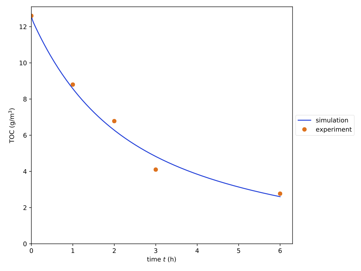
In the same folder, you find the raw data files with corresponding units.
The saved plot shows the TOC development over time compared to the experimental results.